In the past, writing simple programs to generate fractal images is something I have found myself returning to over and over again. I’ve done it so many times that I can probably write a Mandelbrot Set generator in my sleep. However, I’ve really struggled to understand at an intuitive level why these shapes emerge the way they do from such deceptively simple looking iterative functions.
Over the recent Christmas break I spent some time playing with Julia Set visualisations. My aim was to gain a better understanding of why these sets often take on exotic fractal shapes. I’ve really stuck with it this time and I finally feel like I’m beginning to gain a better understanding. Today, I finally feel like I’ve achieved a bit of a breakthrough in my own understanding, which I’ll try to illustrate in the following images.


The solid black shape in each image is the so-called filled Julia Set of a complex iterating function, f. Specifically, in the images above,

where z and c are complex values and c = 0.325 + 0.285j. Different values of c produce very different shapes. The basic idea is that for a given value of c you select an initial value of z – let’s call it z0 – and then apply the iterating function f over and over again to generate a sequence of complex values
where
We call this sequence the orbit of z0 under f. For the function f shown above, every point in the complex plane falls into one of three possible categories:
- The points which are coloured white in the images above have orbits which spiral out to infinity. These points make up F0, one of the Fatou domains of f.
- The points which are coloured black in the images above have orbits which remain bounded (they stay within the black region). These points make up F1, the second Fatou domain of f.
- The third category is the set of points which form the boundary between the two Fatou domains – this is the Julia Set of f. In the images above, the Julia Set is basically where the black region meets the white region. The orbit of any point in the Julia Set lies completely within the Julia Set – i.e. the orbit just jumps around the boundary forever, never going inside or outside.
The Julia Set of this function has a fractal shape, as is the case for many complex functions. What I’m really trying to understand – in an intuitive sense – is why that is the case. Self-similarity is a frequently mentioned characteristic of fractals – specifically the recurrence of similar shapes within the fractal at different levels of magnification. There’s no doubt that very similarly shaped outcrops appear repeatedly along the boundary of the filled Julia sets shown above. Furthermore, if we were to zoom into that boundary, we would see identically shaped outcrops recurring over and over again at different levels of magnification.
The insight that struck me so forcefully today relates to picturing how the iterating function generates this self-similarity. In the image on the left, the green dot marks the location of z0 in the complex plane. The orbit of z0 is shown as a series of red dots joined by blue lines which illustrate what happens to z each time the function is iterated (first z is squared which is represented by the curve, then c is added to it which is represented by the straight line). When I traced z0 along just outside the boundary, I could see z1, z2, z3, etc tracing out similar shapes further up the boundary. The best way I can describe it is that it reminded me of a pantograph, but with many pens rather than just one.
The images above are screen shots of a python program (“julia.py”) I wrote to display filled Julia sets and visualise the orbits of different complex numbers. The complete Python code is shown below. To run this, I think you just need Python and Tkinter. I’m running Python 2.7.9, but hopefully it should work in Python 3 also (?). Basic instructions are below the code listing.
#
# julia.py - Real time orbit viewer for iterative complex functions
# written by Ted Burke, last updated 21-1-2016
#

from Tkinter import *
import math
import sys

def generate_fractal():
    sys.stdout.write('Generating fractal for c = {:.3f} + {:.3f}j...'.format(c.real,c.imag))
    sys.stdout.flush()
    for y in range(h):
        for x in range(w):
            z = centre + complex(((x-(w-1)/2.0)*pxw),(((h-1)/2.0-y)*pxw))
            n = 0
            while abs(z) < limit and n < 51:
                try:
                    z = pow(z,a) + c
                    n = n + 1
                except ZeroDivisionError:
                    z = limit
            pixel = int(255 * (0.5 + 0.5*math.cos(math.pi*n/51.0)))
            img.put('#{:02x}{:02x}{:02x}'.format(pixel,pixel,pixel),(x,y))
    sys.stdout.write('OK\n')
    sys.stdout.flush()

def set_z0(event):
    global z0
    z0 = complex((event.x - w/2) * pxw, (h/2 - event.y) * pxw)
    paint()

def set_c(event):
    global c
    c = complex((event.x - w/2) * pxw, (h/2 - event.y) * pxw)
    generate_fractal()
    paint()

def paint():
    canv.delete("all")
    canv.create_rectangle(0, 0, w, h, fill="white")
    canv.create_image((0,0), anchor="nw", image=img, state="normal")
    z = z0
    x = int(w/2 + z.real/pxw)
    y = int(h/2 - z.imag/pxw)
    canv.create_oval(x-3,y-3,x+4,y+4,fill="green")
    for n in range(100):
        p1 = z
        for m in range(M+2):
            if m<=M:
                p2 = pow(z,1.0+((a-1.0)*m)/M)
            else:
                p2 = p2 + c
            x1 = int(w/2 + p1.real / pxw)
            y1 = int(h/2 - p1.imag / pxw)
            x2 = int(w/2 + p2.real / pxw)
            y2 = int(h/2 - p2.imag / pxw)
            canv.create_line(x1, y1, x2, y2, fill="blue")
            p1 = p2
        z = pow(z,a) + c
        x = int(w/2 + z.real/pxw)
        y = int(h/2 - z.imag/pxw)
        canv.create_oval(x-3,y-3,x+4,y+4,fill="red")
        if (abs(z) > 10): break

# Create master Tk widget
master = Tk()
master.title('Julia Set Explorer - by Ted Burke - see http://batchloaf.com')

# Dimensions and resolution
w,h = 800,800
centre = 0 + 0j
pxw = 0.005

# Create Tk canvas widget
canv = Canvas(master, width=w, height=h)
canv.pack()
canv.bind("<B1-Motion>", set_z0)
canv.bind("<Button-1>",  set_z0)
canv.bind("<Button-2>",  set_c)
canv.bind("<Button-3>",  set_c) # this is actually the right click

# Iterating function parameters
a = 2.0
c = 0.325 + 0.285j
z0 = 0 + 0j
limit = 10

# Number of steps in plotting each curve within each orbit
M = 40

# Create image object to store Julia Set image
img = PhotoImage(width=w, height=h)

# Generate initial Julia Set image
generate_fractal()
paint()

# Main Tk event loop
mainloop()
To use the program,
- Left click anywhere on the image to set the value of z0, which will update the displayed orbit.
- Clicking and dragging will update z0 and its orbit in real time, which really helps to see what’s going on.
- Right click anywhere on the image to set c, which will updated the background filled Julia Set image (the black shape). It takes a little time to generate the new image, so be patient!
I’m running Xubuntu 15.04 Linux here, so Python 2.7.9 was already installed by default. I needed to install Tkinter though, which is Python’s standard GUI toolkit. To install Tkinter, I just did
sudo apt-get install python-tk

